Integer Triangle Traits
Julia Implementation
Part III

Outline

Orthogonal Polynomials
The Catalan Triangles
Traits of Catalan's aerated Δ
The normalized Catalan Triangle
The extended Catalan Triangle
The Motzkin Triangle
The traits of Motzkin's Δ
Deléham's Delta operator
The Schröder triangles
The traits of the Big-Schröder triangle
The Little-Schröder triangle
Riordan squares
The origin of a triangle
The Jacobsthal triangle
The traits of Jacobsthal triangle
The traits of Fibonacci triangle
Outlook

In three parts, we want to consider how the programming language Julia can be applied in the study of integer sequences, in particular of integer triangles.

In the first part, we put together some basic terminology and concepts.
In the second part we examine the connection with polynomial sequences.
The third part deals with general algorithms for constructing integer triangles.

The article is written in the hope of making it easier for friends of number sequences (SeqFans) to get started with the Julia language. And conversely, that it might animate one or the other member of the Julia community to write contributions for the OEIS. It can also be read as an introductory tutorial to the registered package "IntegerTriangle".

We choose Julia because it is currently (2020) the language best suited for many tasks in scientific computing and, equally important, is an elegant language that makes coding fun. As one co-creator of Julia puts it: "Julia was designed to help researchers write high-level code in an intuitive syntax and produce code with the speed of production programming languages."

Julia is free and open-source. We use version 1.4 which was released in 2020. This article and the code is available under the Creative Commons Attribution 3.0 license.

Orthogonal Polynomials

Sequences of polynomials over ℤ are the natural conceptualization of integer triangles, so it suggests itself to consider the important subclass of orthogonal polynomials.

By the theorem of Favard an orthogonal polynomial systems p_n(x) is a sequence of real polynomials with deg(p_n(x)) = n for all n if and only if

     p_n+1(x) = (x - s_n)p_n(x) - t_n p_n-1(x)

with p₀(x) = 1 for some pair of sequences s_n and t_n.

The next function implements Favard's theorem and returns the coefficients of the polynomials as an integer triangle with dim rows.

DEF:  function OrthoPoly(dim::Int, s::Function, t::Function)
          T = ℤTriangle(dim, reg=true)
          for n ∈ 1:dim T[n][n] = ℤInt(1) end
          for n ∈ 2:dim
              u(k) = k == 0 || k == n ? 0 : T[n-1][k]
              for k ∈ 1:n-1
                  T[n][k] = u(k-1) + s(k-1)*u(k) + t(k)*u(k+1)
              end
          end
          T
      end

Now that the machinery has been set up and we can concentrate on the functions s and t that produce classic orthogonal polynomials (or invent new ones).

The Catalan Triangles

There are many variants of the Catalan triangle in the OEIS, we consider here the three main variants, which are intimately connected.

The aerated Catalan triangle, Lang's A053121.
The normalized Catalan triangle, Bower's A033184.
The extended Catalan triangle, Luschny's A189231.

The aerated Catalan is the basic variant and arguably the most important one. It has a 3-term recursion, which qualifies the Catalan numbers as coefficients of orthogonal polynomials.

DEF:  Catalan(dim) = OrthoPoly(dim, n -> 0, n -> 1)

IN:   Catalan(7)
OUT:  Array{fmpz,1}
      [[1],
      [0, 1],
      [1, 0, 1],
      [0, 2, 0, 1],
      [2, 0, 3, 0, 1],
      [0, 5, 0, 4, 0, 1],
      [5, 0, 9, 0, 5, 0, 1]]

The aerated Catalan Triangle.

Traits of Catalan's aerated Δ

Catalan:     1, 0, 1, 1, 0, 1, 0, ...  A053121  Lang      2000
InvCatalan:  1, 0, 1,-1, 0, 1, 0, ...  A049310  Lang      1999
DiagCatalan: 1, 0, 1, 1, 0, 0, 2, ...  missing*
PolyCatalan: 1, 0, 1, 1, 1, 1, 0, ...  A330608  Luschny   2020
--
Sum:       1, 1, 2, 3, 6, 10, 20, ...  A001405  Sloane    1973
EvenSum:   1, 0, 2, 0, 6, 0, 20, ...   A126869  Deléham   2007
OddSum:    0, 1, 0, 3, 0, 10, 0, ...   A138364 Sutherland 2008
AltSum:    1, -1, 2, -3, 6, -10, ...   A126930  Deléham   2007
DiagSum:   1, 0, 2, 0, 5, 0, 14, ...   A126120* Deléham   2007
Central:   1, 0, 3, 0, 20, 0, 154, ... A126596* Deléham   2007
LeftSide:  1, 0, 1, 0, 2, 0, 5, 0, ... A126120  Deléham   2007
RightSide: 1, 1, 1, 1, 1, 1, 1, 1, ... A000012  Sloane    1994
PosHalf:   1, 1, 5, 9, 45, 97, 485, .. A121724  Barry     2007
NegHalf:   1, 1, 5, 9, 45, 97, 485, .. A121724  Barry     2007
N0TS:      0, 1, 2, 5, 10, 22, 44, ... A045621  Bloom     1999
NATS:      1, 2, 4, 8, 16, 32, 64, ... A000079  Sloane    1973
--
missing* DiagCatalan is A033184 with the zero-rows.
A126120* is A126120 shifted left twice.
A126596* aerated version of A126596.

The normalized Catalan Triangle

Consider first the diagonalized form of the aerated Catalan triangle:

IN:   DiagonalTriangle(Catalan(9))

OUT:  Array{fmpz,1}
      [1]
      [0]
      [1, 1]
      [0, 0]
      [2, 2, 1]
      [0, 0, 0]
      [5, 5, 3, 1]
      [0, 0, 0, 0]
      [14, 14, 9, 4, 1]

The diagonalized form of the aerated Catalan triangle.

The normalized Catalan triangle is the diagonalized form of the aerated Catalan triangle with the all-zero rows deleted.

T(n,k) = ((k+1)(2n-k)!)/((n-k)!(n+1)!)

This is A033184 based in (0,0). Note that we prefer it to its row reversed form, Meeussen's A009766 (which seems to be more popular) because it allows the starting point, the aerated triangle, to be invertible. And by this, it exhibits the connection to Chebyshev's U polynomials given by Lang's A049310.

The extended Catalan Triangle

Instead of deleting the zeros from the aerated Catalan triangle and the zero rows from its diagonalized form, we can try to fill the 'holes' in a meaningful way. (The feeling that zero is not a number equal to the others, that its appearance indicates a gap, is a centuries-old cultural phenomenon in Western intellectual history that has not been changed even by modern mathematics.)

One way to do so might be called CatalanBallot and the triangle itself extended Catalan triangle. We implement it as a recurrence with a cache.

DEF: const CacheBallot = Dict{Tuple{Int,Int},fmpz}()

     function CatalanBallot(n::Int, k::Int)
        haskey(CacheBallot, (n,k)) && return CacheBallot[(n,k)]
        (k > n || k < 0) && return ℤInt(0)
        n == k && return ℤInt(1)
        CacheBallot[(n, k)] = (
            CatalanBallot(n - 1, k - 1) +
            CatalanBallot(n - 1, k + 1) +
            (iseven(n - k) ? 0 : CatalanBallot(n - 1, k))
        )
     end

     CatalanBallot(n) = [CatalanBallot(n, k) for k ∈ 0:n]

IN:   CatalanBallot.(0:6) |> println

OUT:  Array{fmpz,1}
      [ 1]
      [ 1,   1]
      [ 1,   2,  1]
      [ 3,   2,  3,   1]
      [ 2,   8,  3,   4,  1]
      [10,   5, 15,   4,  5,  1]
      [ 5,  30,  9,  24,  5,  6, 1]

The extended Catalan Triangle.

Someone made the joke that Catalan lost half of his numbers because he used the ternary operator in his calculations but confused the odd and even case. If you don't understand the joke, you have to look closer at the above function.

More seriously, the idea behind this version is to exchange the central binomial in the well-known formula of the Catalan numbers with the swinging factorial, which is a generalization of the central binomial. This frees the binding of the Catalan numbers to the even case, which is obviously generated by the central binomial coefficient.

The Motzkin Triangle

The simplest case in the Favard setup of orthogonal polynomials is s(n) = 1 and t(n) = 1. This leads to the Motzkin polynomials.

DEF:  Motzkin(dim) = OrthoPoly(dim, n -> 1, n -> 1)

IN:   Motzkin(7)
OUT:  Array{fmpz,1}
      [[1],
      [ 1,  1],
      [ 2,  2,  1],
      [ 4,  5,  3,  1],
      [ 9, 12,  9,  4,  1],
      [21, 30, 25, 14,  5, 1],
      [51, 76, 69, 44, 20, 6, 1]]

The Motzkin Triangle.

In the OEIS, this is called the Motzkin triangle in reverse order, but this is not the best way. In this and similar cases we prefer a set up where the right side of the triangle is the identity, and the left side is the sequence which gives its name to the triangle.

The traits of Motzkin's Δ

 Motzkin:     1, 1, 1, 1, 2, 1, 1, ...  A064189  Sloane     2001
 InvMotzkin:  1, -1, 1, 0, -2, 1, ...   A104562  Barry      2005
 DiagMotzkin: 1, 1, 2, 1, 4, 2, 9, ...  A106489* Deutsch    2005
 PolyMotzkin: 1, 1, 1, 2, 2, 1, 4, ...  A330792  Luschny    2020
 --
 Sum:       1, 2, 5, 13, 35, 96, ...    A005773* Sloane     1991
 EvenSum:   1, 1, 3, 7, 19, 51, ...     A002426  Sloane     1973
 OddSum:    0, 1, 2, 6, 16, 45, ...     A005717* Sloane     1991
 AltSum:    1, 0, 1, 1, 3, 6, 15, ...   A005043  Sloane     1991
 DiagSum:   1, 1, 3, 6, 15, 36, 91, ... A005043* Sloane     1991
 Central:   1, 2, 9, 44, 230, 1242, ... A026302  Kimberling 1999
 LeftSide:  1, 1, 2, 4, 9, 21, 51, ...  A001006  Sloane     1973
 RightSide: 1, 1, 1, 1, 1, 1, 1, 1, ... A000012  Sloane     1994
 PosHalf:   1, 3, 13, 59, 285, ...      A330799  Luschny    2020
 NegHalf:   1, -1, 5, -17, 77, ...      A330800  Luschny    2020
 N0TS:      0, 1, 4, 14, 46, 147, ...   A330796	 Luschny    2020
 NATS:      1, 3, 9, 27, 81, 243, ...   A000244	 Sloane     1973
 --
 A106489* = A106489 with offset 0
 A005773*(n) = A005773(n+1)
 A005717* = (0) + A005717
 A005043*(n) = A005043(n+2)

It is interesting that the diagonal sum DiagSum here is the alternating sum AltSum shifted to the left twice.

Deléham's Delta operator

A clever way to associate two generating functions with bivariate polynomials and then evaluate them row by row was introduced by Philippe Deléham in 2003 in a submission to the OEIS (A084938). His method was later studied by Paul Barry and Richard J. Mathar but has not yet found the attention in the standard literature that it deserves. Our implementation is a simplified version that uses only univariate polynomials.

DEF:  function DeléhamΔ(dim::Int, s::Function, t::Function)
          T = ℤTriangle(dim)
          ring, x = ℤPolyRing("x")
          A = [s(k) + x * t(k) for k ∈ 0:dim-2]
          C = fill(ring(1), dim + 1); C[1] = ring(0)
          m = 1
          for k ∈ 0:dim-1
              for j ∈ k+1:-1:2
                  C[j] = C[j-1] + C[j+1] * A[j-1]
              end
              T[m] = [coeff(C[2], j) for j ∈ 0:k]
              m += 1
          end
          T
      end

Some examples are:

[1, 2, 3, 4, 5, 6, 7, ...] Δ [1, 0, 0, 0, 0, 0, 0, ...]
A321627, related to the double factorial of odd numbers.

[1, 4, 9, 16, 25, 36, 49, ...] Δ [1, 0, 0, 0, 0, 0, ...]
A321630, related to the Euler numbers.

[1, 0, 0, 0, 0, 0, ...] Δ [0, 1, 2, 2, 3, 3, ...]
A263484, related to the connectivity set of permutations.

[1, 2, -5/2, 1/2, 0, 0, 0, ...] Δ [1, 0, 0, 0, 0, ...]
A321624, related to the the Lucas numbers.

[1, 1, 2, 1, 2, 1, 2, 1, ...] Δ [1, 0, 0, 0, 0, ...]
A321623, related to the large Schröder numbers.

The Schröder triangles

Let's compute the Big-Schröder triangle with Deléham's Delta, which, according to our taxonomy and conventions, is triangle A080247 in the OEIS. There it bears the terrible and obfuscating name "Formal inverse of triangle A080246. Unsigned version of A080245".

IN:   s(n) = iszero(n) ? 1 : isodd(n) ? 1 : 2
      BSchröder(dim) = DeléhamΔ(dim, s , n -> 0^n)
      BSchröder(7) |> println

OUT:  Array{fmpz,1}
     [[   1],
      [   2,    1],
      [   6,    4,   1],
      [  22,   16,   6,   1],
      [  90,   68,  30,   8,  1],
      [ 394,  304, 146,  48, 10,  1],
      [1806, 1412, 714, 264, 70, 12, 1]]

The Big-Schröder Triangle.

The traits of the Big-Schröder triangle.

Triangle:  1, 2, 1, 6, 4, 1, 22,...    A080247  Barry     2003
InvTria:   1, -2, 1, 2, -4, 1, -2, ... A080246  Barry     2003
Diag       1, 2, 6, 1, 22, 4, 90, ...  missing
PolyVal                                missing
--
Sum:       1, 3, 11, 45, 197, 903, ... A001003* Sloane    1973
EvenSum:   1, 2, 7, 28, 121, 550,  ... A010683  Sulanke   1999
OddSum:    0, 1, 4, 17, 76, 353,  ...  A239204* Kruchinin 2014
AltSum:    1, 1, 3, 11, 45, 197, ...   A001003  Sloane    1973
DiagSum:   1, 2, 7, 26, 107, 468, ...  A006603  Sloane    1991
Central:   1, 4, 30, 264, 2490, ...    A330801  Luschny   2020
LeftSide:  1, 2, 6, 22, 90, 394, ...   A006318  Sloane    1991
RightSide: 1, 1, 1, 1, 1, 1, 1, ...    A000012  Sloane    1994
PosHalf:   1, 5, 33, 253, 2121, ...    A330802  Luschny   2020
NegHalf:   1, -3, 17, -123, 1001, ...  A330803  Luschny   2020
N0TS:      0, 1, 6, 31, 156, 785, ...  A065096  Meeussen  2001 
NATS:      1, 4, 17, 76, 353, 1688, .. A239204  Kruchinin 2014 
--
A001003* = A001003 shifted left once
A239204* = (0) + A239204

The Little-Schröder triangle

Next, what about little Schröder?

IN:   s(n) = isodd(n) ? 2 : 1
      LSchröder(dim) = DeléhamΔ(dim, s , n -> 0^n)
      LSchröder(7) |> println

OUT:  Array{fmpz,1}
      [[ 1],
      [  1,    1],
      [  3,    4,    1],
      [ 11,   17,    7,   1],
      [ 45,   76,   40,  10,  1],
      [197,  353,  216,  72,  13,  1],
      [903, 1688, 1145, 458, 113, 16, 1]]

The little-Schröder Triangle.

In this setup the generating input for the big-Schröder triangle differs from the input for the little-Schröder triangle only in a single value: s(0) = 0 in the first case but s(0) = 1 in the latter case.

If we look at the traits of the triangle, then we see that the alternating rows sum to <1,0,0,0,…>. That's a clue! The triangle might be a Riordan square.

Riordan squares

The Riordan square is a sequence−to−triangle transformation. Given the sequence a,b,c,... the first few rows of the triangle are:

The Riordan Square of a, b, c, d, e, ...
a
b	ab
c	ac+b²	ab²
d	ad+2bc	b(b²+2ac)	ab³
e	ae+2bd+c²	2abd+ac²+3cb²	b²(b²+3ac)	ab⁴

We call the sequence a,b,c,... the generating sequence of the Riordan square. Further we require that a ≠ 0, b ≠ 0. Note that this implies that if p_n denote the polynomials which are associated with a Riordan square than degree(p_n(x)) = n (∀ n ≥ 0).

In the further course we assume that a = 1 and b = 1, for the obvious reason to make all entries on the right side 1. Then the associated polynomials are monic and their constant coefficient is the n-th term of the generating sequence of the triangle. This simplifies the triangle to:

The Riordan Square of 1, 1, c, d, e, ...
1
1	1
c	c+1	1
d	d+2c	2c+1	1
e	e+2d+c²	2d+3c+c²	3c+1	1

In this form the Riordan square has an inverse, which starts:

The inverse Riordan Square of 1, 1, c, d, e, ...
1
-1	1
1	-c-1	1
-1	-d+c+2c²+1	-1-2c	1
1	-e+d-2c²+5dc-c-5c³-1	-2d+2c+5c²+1	-3c-1	1

And finally the general case, where we generate the sequence by a function f. As always, the evalution of the function starts at n = 0.

DEF: function RiordanSquare(dim::Int, f::Function)
        T = ℤTriangle(dim, reg=true)
        for n ∈ 0:dim-1 T[n+1][1] = f(n) end
        for k ∈ 1:dim-1, m ∈ k:dim-1
            T[m+1][k+1] = sum(T[j][k]*T[m-j+2][1] for j ∈ k:m)
        end
        T
    end

The RiordanSquare has a second form, the exponential Riordan square. This form is associated with a bivariate exponential generating function and normalizes the Riordan square for this case.

DEF: function ExpRiordanSquare(dim::Int, s::Function)
        R = RiordanSquare(dim, s)
        for k ∈ 1:dim-1
            u *= k
            for m ∈ 1:k
                j = (m == 1 ? u : div(j, m-1))
                R[k+1][m] *= j
            end
        end
        R
    end

The origin of a triangle

The first thing to observe is that the alternating row sums of a Riordan square build the sequence 1,0,0,..., i.e. all nonconstant polynomials generated by Riordan squares vanish in x = -1.

We have by now defined 16 characteristics of a triangle, 4 triangles (2-dim) and 12 sequences (1-dim). Now we add a 0-dim characteristic: If the polynomials associated with a triangle, with the exception of the constants, all disappear in one point, then we say the triangle has its origin in this point.

For example the standard polynomials x^n have the origin (0, 0), the Eulerian polynomials have origin (0, 1) and the Jacobsthal polynomials the origin (-1, 0).

The Jacobsthal polynomials.

The Jacobsthal triangle

The Jacobsthal triangle is the Riordan square with the generating sequence J(n) = J(n-1) + 2*J(n-2) and initial values a(n) = 1 for n ≤ 2 .

DEF:  Jacobsthal(dim) = RiordanSquare(dim, J)

In:   Jacobsthal(7)
OUT:  Array{fmpz,1}
      [[ 1],
      [  1,   1],
      [  1,   2,  1],
      [  3,   5,  3,  1],
      [  5,  12, 10,  4,  1],
      [ 11,  27, 28, 16,  5, 1],
      [ 21,  62, 75, 52, 23, 6, 1]]

The traits of Jacobsthal triangle

Triangle:  1, 1, 1, 1, 2, 1, 3, 5, ...  A322942  Luschny 2019
InvTria:   1, -1, 1, 1, -2, 1, -1, ...  A330794  Luschny 2020
DiagTria:  1, 1, 1, 1, 3, 2, 5, 5, ...  missing
PolyVal:                                missing
--
Sum:       1, 2, 4, 12, 32, 88,  ...    A152035  Bagula  2008
EvenSum:   1, 1, 2, 6, 16, 44, 120, ... A002605* Mallows 1996
OddSum:    0, 1, 2, 6, 16, 44, 120, ... A002605  Mallows 1996
AltSum:    1, 0, 0, 0, 0, 0, 0, 0, ...  A000007  Sloane  1994
DiagSum:   1, 1, 2, 5, 11, 26, 59, ...  A006138* Sloane  1991
Central:   1, 2, 10, 52, 290, 1706, ... A166694  Barry   2009
LeftSide:  1, 1, 1, 3, 5, 11, 21, ...   A152046  Bagula  2008
RightSide: 1, 1, 1, 1, 1, 1, 1, 1, ...  A000012  Sloane  1994
PosHalf:   1, 3, 9, 51, 225, 1083, ...  A323232	 Luschny 2019
NegHalf:   1, -1, 1, -9, 17, -89, ...   A015443* Gérard  1999
N0TS:      0, 1, 4, 14, 48, 156, ...    A331319  Luschny 2020 
NATS:      1, 3, 8, 26, 80, 244, ...    A331320  Luschny 2020
--
A002605* = A002605 with a(0) = 1.
A006138* = (1) + A006138.
A152046 = A001045 with a(0) = 1.
A015443* = (1) + signed(A015443).
--

What happens if we drop the factor 2 in the above reccurence? More precicely, we define:

DEF: FJ(n, k) = n <= 2 ? 1 : FJ(n-1, k) + k*FJ(n-2, k)
     FibonacciTriangle(dim)  = RiordanSquare(dim, n -> FJ(n,1))
     JacobsthalTriangle(dim) = RiordanSquare(dim, n -> FJ(n,2))

Of course the function FJ(n, k) needs a better implementation, for example by using a cache. Here the point to observe is that FJ(0,k) = 1.

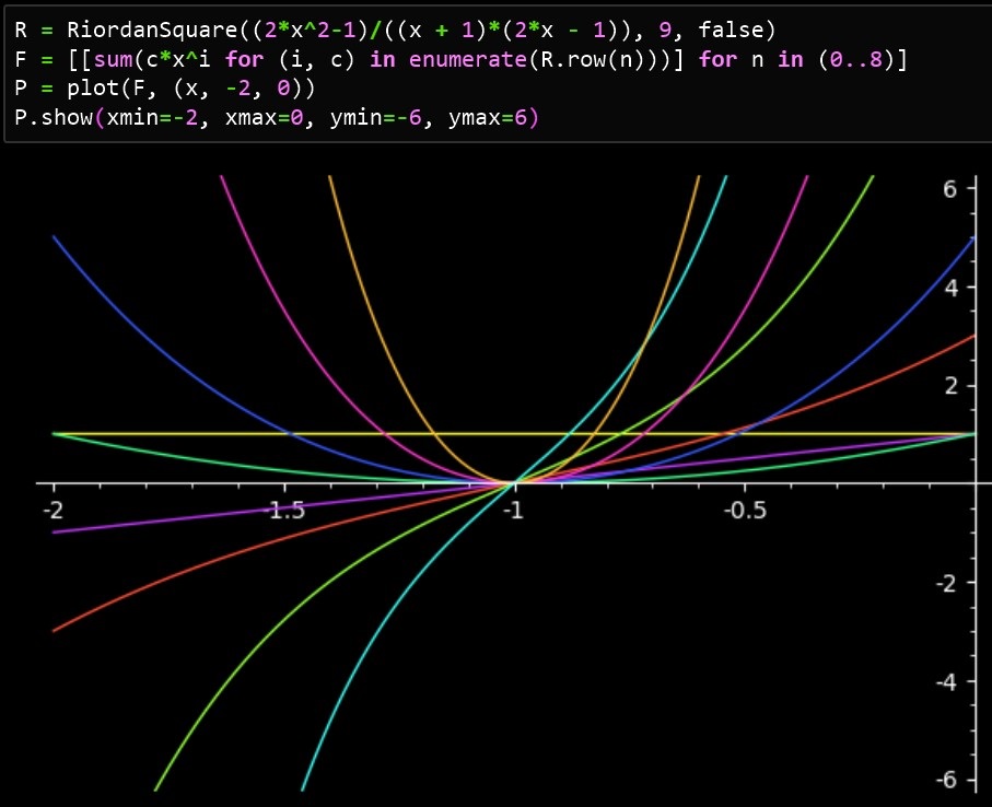
The Jacobsthal sequence with a(0)=1 is Bagula's A152046 and has the Riordan square A322942. The Fibonacci sequence with a(0)=1 is Wiseman's A324969 with offset 0 and has the Riordan square A193737. The profile of this triangle is shown below.

The traits of Fibonacci triangle

 Triangle:  1, 1, 1, 1, 2, 1, 2, 4, ...   A193737 Kimberling 2011
 InvTria:   1, -1, 1, 1, -2, 1, -1, ...   missing
 DiagTria:  1, 1, 1, 1, 2, 2, 3, 4, ...   A119473* Deutsch   2006
 PolyVal:                                 missing 
 --
 Sum:       1, 2, 4, 10, 24, 58, 140, ... A052542  ECS*      2000
 EvenSum:   1, 1, 2, 5, 12, 29, 70, ...   A215928  Somos     2012
 OddSum:    0, 1, 2, 5, 12, 29, 70, ...   A215928* Somos     2012
 AltSum:    1, 0, 0, 0, 0, 0, 0, 0, ...   A000007  Sloane    1994
 DiagSum:   1, 1, 2, 4, 8, 16, 32, ...    A011782  Killough  1996
 Central:   1, 2, 8, 36, 170, 826, ...    A330793  Luschny   2020
 LeftSide:  1, 1, 1, 2, 3, 5, 8, 13, ...  A324969* Wiseman   2019
 RightSide: 1, 1, 1, 1, 1, 1, 1, 1, ...   A000012  Sloane    1994
 PosHalf:   1, 3, 9, 39, 153, 615, ...    A330795  Luschny   2020
 NegHalf:   1, -1, 1, -5, 9, -29, ...     A006131* Sloane    1995
 N0TS:      0, 1, 4, 13, 40, 117, ...     A119915  Deutsch   2006
 NATS:      1, 3, 8, 23, 64, 175, ...     A331321  Luschny   2020
 --
 A119473* = 1 + A119473
 ECS* = INRIA Algorithms Project.
 A215928* = A215928 with a(0)=1 <-> a(0)=0.
 A324969* = A324969 with offset 0.
 A006131* = 1 + (-1)^n*A006131

Outlook

Perhaps the reader has already wondered what the profiles of the Stirling numbers look like. In the next installment of this series, we will discuss Julia's important iteration protocol. Based on this protocol, we will define a whole class of triangles, the most prominent of which are the two Stirling number triangles. So stay tuned and have fun coding with Julia!

Here we already give a preview of the trait cards of the Stirling triangles and the Euler triangle.


🔶  Stirling Set Numbers

Trait       Seq                              Anum      Author      Year
----------  -------------------------------  --------  ----------  ----
Δ Triangle  1, 0, 1, 0, 1, 1, 0, 1, 3, ...   A048993   Sloane      1999
Δ Inverse   1, 0, 1, 0, -1, 1, 0, 2, ...     A048994   Sloane      1999
Δ Diagonal  1, 0, 0, 1, 0, 1, 0, 1, 1, ...   A136011*  Adamson     2007
Δ Polynom   1, 0, 1, 0, 1, 1, 0, 2, 2, ...   A189233   Luschny     2011 
Sum         1, 2, 5, 15, 52, 203, 877, ...   A000110   Sloane      1973
EvenSum     1, 1, 2, 7, 27, 106, 443, ...    A024430   Kimberling  1999
OddSum      0, 1, 3, 8, 25, 97, 434, ...     A024429   Kimberling  1999
AltSum      1, 0, -1, -1, 2, 9, 9, ...       A000587   Sloane      1973
DiagSum     1, 1, 2, 4, 9, 22, 58, ...       A171367   Barry       2009
Central     1, 3, 25, 350, 6951, ...         A007820   Kemp        1996
LeftSide    1, 0, 0, 0, 0, 0, 0, 0, 0, ...   A000007   Sloane      1994
RightSide   1, 1, 1, 1, 1, 1, 1, 1, 1, ...   A000012   Sloane      1994
PosHalf     1, 1, 3, 11, 49, 257, 1539, ...  A004211   Sloane      1991
NegHalf     1, 1, -1, -1, 9, -23, -25, ...   A009235   Hardin      1996
N0TS        0, 1, 3, 10, 37, 151, 674, ...   A005493*  Sloane      1991
NATS        1, 2, 5, 15, 52, 203, 877, ...   A000110*  Sloane      1973

A136011* without the first column of A048993.
A005493* = (0) + A005493.
A000110* = A000110 shifted left once.


🔶  Stirling Cycle Numbers
    
Trait       Seq                              Anum      Author    Year
----------  -------------------------------  --------  --------- ----
Δ Triangle  1, 0, 1, 0, 1, 1, 0, 2, 3, ... A132393   Deléham   2007
Δ Inverse   1, 0, 1, 0, -1, 1, 0, 1, -3, . A048993*  Sloane    1999
Δ Diagonal  1, 0, 0, 1, 0, 1, 0, 2, 1, ... A331327   Luschny   2020
Δ Polynom   1, 0, 1, 0, 1, 1, 0, 2, 2, ... T265609*  Luschny   2015
Sum         1, 2, 6, 24, 120, 720, 5040, . A000142*  Sloane    1973
EvenSum     1, 0, 1, 3, 12, 60, 360, ...   A001710*  Sloane    1973
OddSum      0, 1, 1, 3, 12, 60, 360, ...   A001710*  Sloane    1973
AltSum      1, -1, 0, 0, 0, 0, 0, 0, ...   A154955*  Granvik   2009
DiagSum     1, 0, 1, 1, 3, 9, 36, 176, ... A237653*  Hanna     2014
Central     1, 1, 11, 225, 6769, 269325,.. A187646   Munarini  2011
LeftSide    1, 0, 0, 0, 0, 0, 0, 0, 0, ... A000007   Sloane    1994
RightSide   1, 1, 1, 1, 1, 1, 1, 1, 1, ... A000012   Sloane    1994
PosHalf     1, 1, 3, 15, 105, 945, ...     A001147   Sloane    1973
NegHalf     1, 1, -1, 3, -15, 105, -945, . A330797   Luschny   2020
N0TS        0, 1, 3, 11, 50, 274, 1764, .. A000254   Sloane    1973
NATS        1, 2, 5, 17, 74, 394, 2484, .. A000774   Sloane    1996
    
A048993* = signed A048993.
T265609* = transpose(A265609)
A000142* shifted left once.
A105752* = unsigned A105752.
A001710* = A001710 with a(1)=0 or a(0)=1.
A154955* = A154955 with offset 0.
A237653* = A237653 shifted left twice.


🔶  Euler Triangle

[0] 1,  
[1] 1,    0,  
[2] 1,    1,     0,  
[3] 1,    4,     1,      0,  
[4] 1,   11,    11,      1,       0,  
[5] 1,   26,    66,     26,       1,       0,  
[6] 1,   57,   302,    302,      57,       1,      0,  
[7] 1,  120,  1191,   2416,    1191,     120,      1,    0,  
[8] 1,  247,  4293,  15619,   15619,    4293,    247,    1,  0,  
[9] 1,  502, 14608,  88234,  156190,   88234,  14608,  502,  1,  0.  


Trait       Seq                          Anum      Author    Year
----------  ---------------------------  --------  --------- ----
Triangle   1, 1, 0, 1, 1, 0, 1, 4, , ... A173018   Sloane    2010 
Δ Inverse  1, -1, 1, 3, -4, 1, -23,  ... A055325*  Bower     2000 
Δ Diagonal 1, 1, 1, 0, 1, 1, 1, 4, 0,... missing   -         -    
Δ Polynom  1, 1, 1, 1, 1, 1, 1, 2, 1,... A332700   Luschny   2020
Sum        1, 1, 2, 6, 24, 120, 720, ... A000142   Sloane    1973 
EvenSum    1, 1, 1, 2, 12, 68, 360, ...  A128103   Stephan   2007 
OddSum     0, 0, 1, 4, 12, 52, 360, ...  A262745   Heinz     2015 
AltSum     1, 1, 0, -2, 0, 16, 0,  ...   A155585   Hanna     2009 
DiagSum    1, 1, 1, 2, 5, 13, 38, , ...  A000800   Harkin    1996 
Central    1, 1, 11, 302, 15619, ...     A180056   Luschny   2010 
LeftSide   1, 1, 1, 1, 1, 1, 1, 1, ...   A000012   Sloane    1994 
RightSide  1, 0, 0, 0, 0, 0, 0, 0, ...   A000007   Sloane    1994 
PosHalf    1, 1, 3, 13, 75, 541, 4683, . A000670   Sloane    1973 
NegHalf    1, 1, -1, -3, 15, 21, -441, . A087674   Jovovic   2003 
N0TS       0, 0, 1, 6, 36, 240, 1800, .  A180119*  Detlefs   2010 
NATS       1, 1, 3, 12, 60, 360,  ...    A001710*  Sloane    1973 

A055325* = inverse of A008292.
A180119* = (0) + A180119.
A001710* = A001710 shifted left once.

Part 1 of the tutorial Part 2 of the tutorial

↻

Integer Triangle Traits Julia Implementation Part III